Control Systems guidelines for Business

When designing or analyzing a system, often it is useful to model the system graphically. Block Diagrams are a useful and simple method for analyzing a system graphically.


The control model uses the transformation process in the context of a technology system

The inputs consist of primary (raw materials) and secondary (energy, manufacturing plant, workforce). There are also primary and secondary output representing the main product and bi-products (worn out staff, spent resources etc) {Source1}

Systems in Series

When two or more systems are in series, they can be combined into a single representative system, with a transfer function that is the product of the individual systems.

If we have two systems, f(t) and g(t), we can put them in series with one another so that the output of system f(t) is the input to system g(t). Now, we can analyze them depending on whether we are using our classical or modern methods.
If we define the output of the first system as h(t), we can define h(t) as:

h(t) = x(t) * f(t)

Now, we can define the system output y(t) in terms of h(t) as:

y(t) = h(t) * g(t)

We can expand h(t):

y(t) = [x(t) * f(t)] * g(t)

But, since convolution is associative, we can re-write this as:

y(t) = x(t) * [f(t) * g(t)]

Our system can be simplified therefore as such:

Series Transfer Functions

If two or more systems are in series with one another, the total transfer function of the series is the product of all the individual system transfer functions.

In the time domain we know that:

y(t) = x(t) * [f(t) * g(t)]

But, in the frequency domain we know that convolution becomes multiplication, so we can re-write this as:

Y(s) = X(s)[F(s)G(s)]

We can represent our system in the frequency domain as:

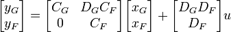
Series State Space

If we have two systems in series (say system F and system G), where the output of F is the input to system G, we can write out the state-space equations for each individual system.
System 1:

x_F' = A_Fx_F + B_Fu

y_F = C_Fx_F + D_Fu

System 2:

x_G' = A_Gx_G + B_Gy_F

y_G = C_Gx_G + D_Gy_F

And we can write substitute these equations together form the complete response of system H, that has input u, and output y_G:

[Series state equation]

[Series output equation]

Systems in Parallel

Blocks may not be placed in parallel without the use of an adder. Blocks connected by an adder as shown above have a total transfer function of:

Y(s) = X(s)[F(s) + G(s)]

Since the Laplace transform is linear, we can easily transfer this to the time domain by converting the multiplication to convolution:

y(t) = x(t) * [f(t) + g(t)]

State Space Model

The state-space equations, with non-zero A, B, C, and D matrices conceptually model the following system:

In this image, the strange-looking block in the center is either an integrator or an ideal delay, and can be represented in the transfer domain as:

or

Depending on the time characteristics of the system. If we only consider continuous-time systems, we can replace the funny block in the center with an integrator:

In the Laplace Domain

The state space model of the above system, if A, B, C, and D are transfer functions A(s), B(s), C(s) and D(s) of the individual subsystems, and if U(s) and Y(s) represent a single input and output, can be written as follows: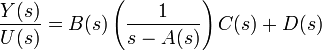

We will explain how we got this result, and how we deal with feedforward and feedback loop structures in the next chapter.

Adders and Multipliers

Some systems may have dedicated summation or multiplication devices, that automatically add or multiply the transfer functions of multiple systems together

Simplifying Block Diagrams

Block diagrams can be systematically simplified.

Transformation		Equation	Block Diagram	Equivalent Block Diagram
1	Cascaded Blocks
2	Combining Blocks in Parallel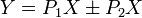
3	Removing a Block from a Forward Loop
4	Eliminating a Feedback Loop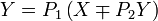
5	Removing a Block from a Feedback Loop
6	Rearranging Summing Junctions
7	Moving a Summing Juction in front of a Block
8	Moving a Summing Juction beyond a Block
9	Moving a Takeoff Point in front of a Block
10	Moving a Takeoff Point beyond a Block
11	Moving a Takeoff Point in front of a Summing Junction
12	Moving a Takeoff Point beyond a Summing Junction

{Source2}

{Source1: http://www.mbanotes.org/node/9 } 
{Source2: http://en.wikibooks.org/wiki/Control_Systems/Block_Diagrams }